2. Solution de référence#
2.1. Méthode de calcul utilisée pour la solution de référence#
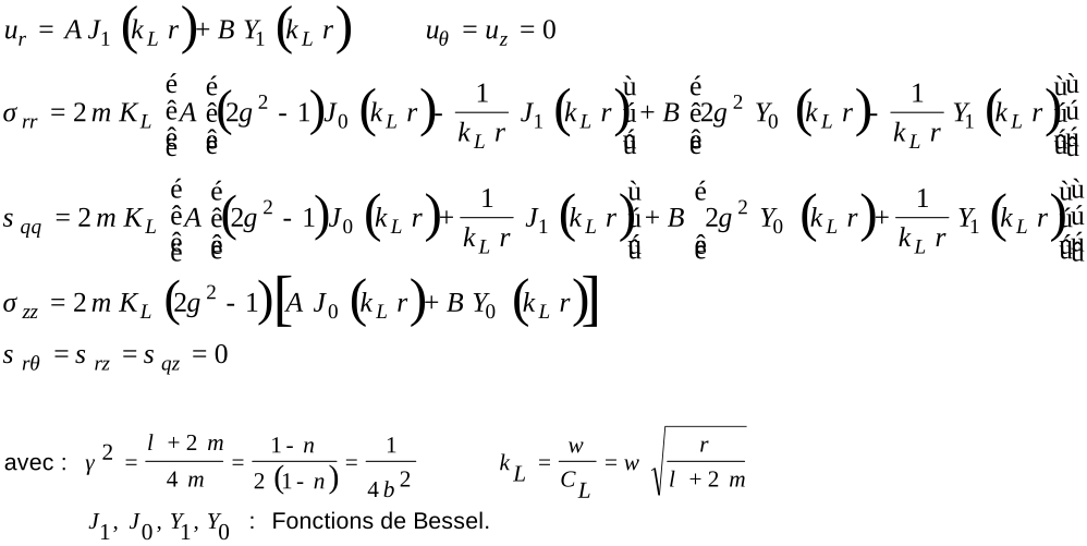
Les constantes \(A\) et \(B\) sont calculées en résolvant le système linéaire obtenu en écrivant :
\({\sigma}_{\mathrm{rr}}(a)=-p\) \({\sigma}_{\mathrm{rr}}(b)=0\)
On obtient :
Pour \(r=0.1\) |
\({u}_{r}=7.3398{10}^{-3}\) |
Pour \(r=0.2\) |
\({u}_{r}=4.6816{10}^{-3}\) |
\({\sigma}_{\mathrm{rr}}=-1\) |
\({\sigma}_{\mathrm{rr}}=0.\) |
||
\({\sigma}_{\theta \theta }=1.6685\) |
\({\sigma}_{\theta \theta }=0.66738\) |
||
\({\sigma}_{zz}=0.20055\) |
\({\sigma}_{zz}=0.20031\) |
Passage dans le système d’axes cartésiens :
\(\begin{array}{ccc}{\sigma}_{xx}& =& {\sigma}_{\mathrm{rr}}{\cos}^{2}\theta +{\sigma}_{\theta \theta }{\sin}^{2}\theta -2{\sigma}_{r\theta }\sin\theta \cos\theta \\ {\sigma}_{yy}& =& {\sigma}_{\mathrm{rr}}{\sin}^{2}\theta +{\sigma}_{\theta \theta }{\cos}^{2}\theta +2{\sigma}_{r\theta }\sin\theta \cos\theta \\ {\sigma}_{xy}& =& {\sigma}_{\mathrm{rr}}\sin\theta \cos\theta -{\sigma}_{\theta \theta }\sin\theta \cos\theta -2{\sigma}_{r\theta }({\cos}^{2}\theta -{\sin}^{2}\theta )\end{array}\)
avec :
\(\theta =0°\) aux points \(A\) et \(B\)
\(\theta =22.5°\) aux points \(C\) et \(D\)
\(\theta =45°\) aux points \(E\) et \(F\)
2.2. Résultats de référence#
Déplacements \((u,v)\) et contraintes
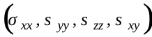
aux points \(A,B,C,D,E,F\) .
2.3. Incertitude sur la solution#
Précision du calcul des Fonctions de Bessel.
2.4. Références bibliographiques#
BONNET : Méthodes des équations intégrales régularisées en élastodynamique- Bulletin de la DER - Série C - N°1/2 - (1987).
ERINGEN - SUHUBI - Elastodynamics, Vol.2 : linear theory Academic Press (1975).