3. Modélisation A#
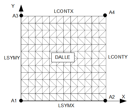
M266
3.1. Caractéristiques du maillage#
Nombre de nœuds : 169
Nombre de mailles et type : 288 TRIA3
3.2. Grandeurs testées et résultats#
Identification |
Type de référence |
Référence |
Tolérance (%) |
\(\mathrm{DZ}(\mathrm{A1})\) |
“ANALYTIQUE” |
2.433 10-4 |
6% |
\(\mathrm{MXX}(\mathrm{A1})\) |
“ANALYTIQUE” |
2% |
|
\(\mathrm{KXX}(\mathrm{A1})\) |
“ANALYTIQUE” |
7.21 10-4 |
5% |
Identification |
Type de référence |
Référence |
Tolérance (%) |
||
\(\mathit{MXX}\) |
\(\mathit{M266}\) |
\(\mathit{Point}3\) |
“NON_REGRESSION” |
4044.16 |
1.e-6 |
\(\mathit{KXX}\) |
\(\mathit{M266}\) |
\(\mathit{Point}3\) |
“NON_REGRESSION” |
7.1996 10-4 |
1.e-6 |
Les grandeurs sont exprimées dans le repère défini par les angles nautiques \(\alpha =33°\) et \(\beta =12°\) .
Identification |
Type de référence |
Référence |
Tolérance (%) |
\(\mathrm{DZ}(\mathrm{A1})\) |
“ANALYTIQUE” |
2.433 10-4 |
6% |
\(\mathit{MXX}(\mathit{A1})\) |
“NON_REGRESSION” |
2847.47 |
1.e-6 |
\(\mathit{MYY}(\mathit{A1})\) |
“NON_REGRESSION” |
1198.15 |
1.e-6 |
\(\mathit{MXY}(\mathit{A1})\) |
“NON_REGRESSION” |
-1852.21 |
1.e-6 |
\(\mathit{KXX}(\mathit{A1})\) |
“NON_REGRESSION” |
5.0692 10-4 |
1.e-6 |
\(\mathit{KYY}(\mathit{A1})\) |
“NON_REGRESSION” |
2.1330 10-4 |
1.e-6 |
\(\mathit{KXY}(\mathit{A1})\) |
“NON_REGRESSION” |
-3.2974 10-4 |
1.e-6 |
Identification |
Type de référence |
Référence |
Tolérance (%) |
||
\(\mathit{MXX}\) |
\(\mathit{M266}\) |
\(\mathit{Point}3\) |
“NON_REGRESSION” |
2842.56 |
1.e-6 |
\(\mathit{MYY}\) |
\(\mathit{M266}\) |
\(\mathit{Point}3\) |
“NON_REGRESSION” |
1197.70 |
1.e-6 |
\(\mathit{MXY}\) |
\(\mathit{M266}\) |
\(\mathit{Point}3\) |
“NON_REGRESSION” |
-1849.40 |
1.e-6 |
\(\mathit{KXX}\) |
\(\mathit{M266}\) |
\(\mathit{Point}3\) |
“NON_REGRESSION” |
5.0605 10-4 |
1.e-6 |
\(\mathit{KYY}\) |
\(\mathit{M266}\) |
\(\mathit{Point}3\) |
“NON_REGRESSION” |
2.1322 10-4 |
1.e-6 |
\(\mathit{KXY}\) |
\(\mathit{M266}\) |
\(\mathit{Point}3\) |
“NON_REGRESSION” |
-3.2924 10-4 |
1.e-6 |
3.3. Remarques#
Les coefficients des matrices d’élasticité suivantes, utilisés lors des calculs, ont été calculés avec \({\nu}_{b}=0\) :
Matrice d’élasticité en membrane : \(\left\lbrace \begin{array}{ccc}4614.& 0& 0\\ 0& 4614.& 0\\ 0& 0& 2142.\end{array}\right\rbrace {10}^{6}N/m\)
Matrice d’élasticité en flexion : \(\left\lbrace \begin{array}{ccc}5.617& 0& 0\\ 0& 5.617& 0\\ 0& 0& 2.57\end{array}\right\rbrace {10}^{6}N/m\)
Pour être certain de rester dans le domaine élastique, les limites élastiques exprimées dans le repère d’orthotropie, sont fixées arbitrairement à une valeur très élevée:
Limites élastiques en flexion positive:
Direction \(x\) : \({1.10}^{10}\mathrm{MNm}/\mathrm{ml}\)
Direction \(y\) : \({1.10}^{10}\mathrm{MNm}/\mathrm{ml}\)
Limites élastiques en flexion négative:
Direction \(x\) : \(–{1.10}^{10}\mathrm{MNm}/\mathrm{ml}\)
Direction \(y\) : \(–{1.10}^{10}\mathrm{MNm}/\mathrm{ml}\)
Comme la structure reste dans le domaine élastique, le coefficient de rappel cinématique (constante de Prager) peut prendre une valeur quelconque.