1. Problème de référence#
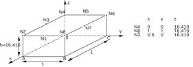
1.1. Géométrie#
1.2. Propriétés de matériaux#
Modélisation A
\(E=1.0\mathrm{MPa}\)
\(\nu =0.3\)
\(k=1.0W/(\mathrm{m.}°C)\)
\({C}_{p}=0J/(°{\mathrm{C.m}}^{3})\)
Modélisation B
\({E}_{L}=1.0\mathrm{MPa}\)
\({E}_{T}=0.9\mathrm{MPa}\)
\({E}_{N}=0.8\mathrm{MPa}\)
\({\nu}_{\text{LT}}=0.1\)
\({\nu}_{\text{LN}}=0.25\)
\({\nu}_{\mathrm{TN}}=0.3333333\)
\(k=1.0W/(\mathrm{m.}°C)\)
\({C}_{p}=0J/(°{\mathrm{C.m}}^{3})\)
1.3. Conditions aux limites et chargements#
Mécanique 3D :
Plan \(z=0\) : |
|
|
Plans \(y=0\) , \(y=1\) : |
\(\mathrm{dy}=0\) |
|
Plans \(x=0\) , \(x=1\) : |
\(\mathrm{dx}=0\) |
|
Nœud : \(O\) |
\(\mathrm{dz}=0\) |
(pour le seul chargement de flexion) |
Chargement : |
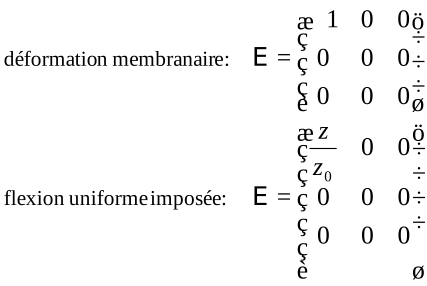
\({z}_{0}=\mathrm{1m}\) |
Mécanique 2D, contraintes planes:
Axe : \(x=0\) Nœud : \(O\) |
\(\mathrm{dx}=0\) \(\mathrm{dy}=0\) |
(ces conditions ne correspondent pas à l’application de la méthode d’homogénéisation). |
Chargement : déformation
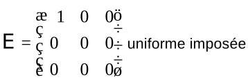
Thermique 3D et 2D:
Plan \(x=0\) |
\(\mathrm{temp}=0\) |
(cette condition ne correspond pas à l’application de la méthode d’homogénéisation). |
Chargement : gradient
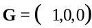
uniforme imposé.