4. Modélisation B

4.1. Géométrie

hauteur: \(h=1m\)

largeur: \(l=1m\)

épaisseur: \(e=1m\)

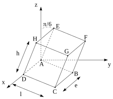
Coordonnées des points (en mètres):

	\(A\)	\(B\)	\(C\)	\(D\)
\(x\)
\(y\)		0.86602540378445	0.86602540378445
\(z\)		–0.5	–0.5

4.2. Caractéristique de la modélisation

3D:

Découpage:1 en hauteur, en largeur et en épaisseur.

Chargement de la phase 1:

Pression de confinement: \(–400\mathit{kPa}\) .

Niveau 3 du modèle CJS

4.3. Caractéristique du maillage

Nombre de nœuds: 8

Nombre de mailles et types: 1 HEXA8 et 6 QUA4

4.4. Grandeurs testées et résultats

Pour confinement: \(–400\mathit{kPa}\)

Localisation	Numéro d’ordre	déformation axiale (%)	contrainte ( \(\mathit{kPa}\) )	Référence	Aster	\(\text{\%}\) différence
Point \(A\)	10	–2.0 %		–400.0	–400.000	< 10–6
	50	–10.0 %		–400.0	–400.000	< 10–6
	100	–20.0 %		–400.0	–400.000	< 10–6
	10	–2.0 %		–53.221	–53.22098	< 10–6
	50	–10.0 %		–63.7665	–63.76653	< 10–6
	100	–20.0 %		–63.7165	–63.71645	< 10–6
	10	–2.0 %		–79.6629	–79.66294	< 10–6
	50	–10..0 %		–111.3	–111.29959	< 10–6
	100	–20.0 %		–111.149	–111.14935	< 10–6
	10	–2.0 %		–22.8994	–22.89941	< 10–6
	50	–10.0 %		–41.1648	–41.16483	< 10–6
	100	–20.0 %		–41.0781	–41.07809	< 10–6