1. Problème de référence#
1.1. Géométrie#
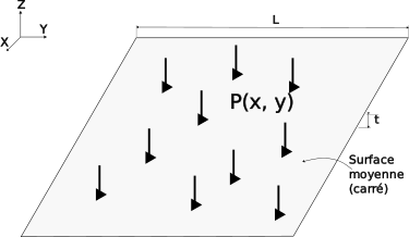
Fig: Schéma du problème de référence
La plaque fine est définie par \(\Omega=[0,L]\times[0,L]\times[-t/2,t/2]\) où
Longueur : \(L = 1 \mathrm{m}\)
Épaisseur : \(t = 0.001 \mathrm{m}\) ou \(t = 0.1 \mathrm{m}\)
1.2. Propriétés de matériaux#
Module d’Young: \(E = 10920 \mathrm{Pa}\)
Coefficient de Poisson: \(\nu = 0.3\)
1.3. Conditions aux limites et chargements#
Encastrement sur le bord (\(w=0\) et \(\theta_x=\theta_y=0\))
Charge surfacique polynomiale :
\[\begin{split}\begin{aligned}
f(x,y) = \frac{E t^{3}}{12 (1 - \nu^{2})}
\Big[
&12 y (y - 1) (5 x^{2} - 5 x + 1) \big(2 y^{2} (y - 1)^{2}\big) \\
&+ x (x - 1) (5 y^{2} - 5 y + 1) \big(2 x^{2} (x - 1)^{2} + 1\big) \\
&+ 12 x (x - 1) (5 y^{2} - 5 y + 1) \big(2 x^{2} (x - 1)^{2}\big) \\
&+ y (y - 1) (5 x^{2} - 5 x + 1) \big(2 y^{2} (y - 1)^{2} + 1\big)
\Big]
\end{aligned}\end{split}\]
1.4. Conditions initiales#
Sans objet pour l’analyse statique.