1. Problème de référence#
1.1. Modélisation A#
1.1.1. Géométrie#
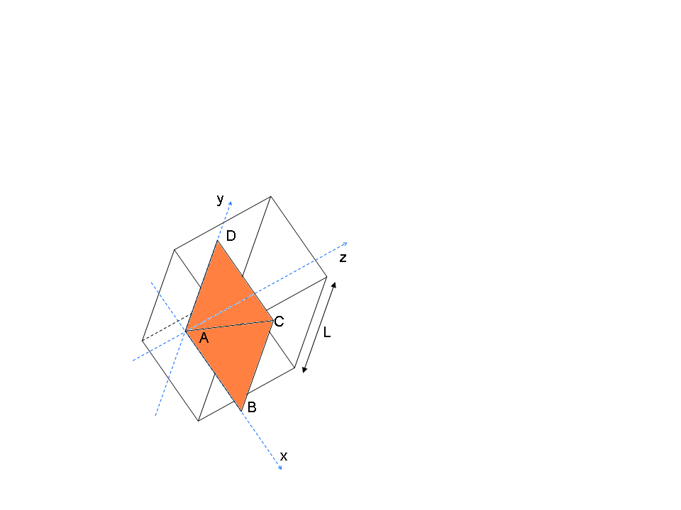
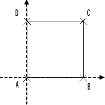
|
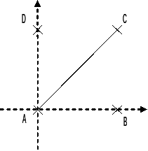
|
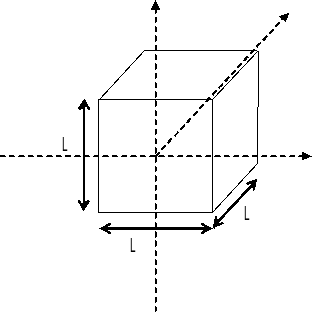
|
\(\mathrm{Carre1}/\mathrm{carre2}\) \(\mathrm{AC}\) \(\mathrm{cube1}\)
Coordonnées des points \((m)\) :
\(A:(0.,0.)\)
\(B:(1.,0.)\)
\(C:(0.,0.)\)
\(D:(0.,1.)\)
Géométrie du cube :
Centre : \((0.,0.,-0.5)\)
Côté : \(L=1\)
Groupe de mailles :
\(\mathrm{carre}1\) surface \(A,B,C,D\)
\(\mathrm{carre}2\) surface \(A,B,C,D\)
\(\mathrm{AC}\) segment \(\mathrm{AC}\)
\(\mathrm{cube1}\) volume
1.1.2. Propriétés du matériau#
Sans objet
1.1.3. Conditions aux limites et chargements#
Sans objet
1.2. Solution de référence#
1.2.1. Méthode de calcul#
Calcul de la référence pour le champ de température
Le champ que l’on projette d’un modèle sur l’autre est un champ analytique de température dont l’évolution est la suivante :
\(T=3.+X+Y\)
La solution de référence est identique au champ analytique projeté.
Calcul de la référence pour le champ de contrainte
L’objectif est d’effectuer un changement de repère, après avoir réalisé une projection d’un champ de contrainte connu sur un maillage vers un maillage 3D.
Passage d’un repère cylindrique (\(\mathrm{XOY}\) ) vers un repère cartésien \(\mathrm{3D}\) (\(\mathrm{XYZ}\) ).
Le champ de contrainte \((N/{m}^{2})\) dans le repère axisymétrique (axe \(\mathrm{OY}\) ) est le suivant:
\(\mathrm{SIXX}=2\)
\(\mathrm{SIYY}=y\)
\(\mathrm{SIZZ}=1\)
\(\mathrm{SIXY}=0.\)
Le champ de contrainte dans le repère cartésien (\(\mathrm{3D}\) ) est obtenu en effectuant :
Une projection du tenseur des contraintes évalué sur le maillage \(\mathrm{2D}\mathrm{axis}\) sur le maillage 3D.
Changement de repère du tenseur des contraintes \([{\sigma}_{\mathrm{3D}}]=[P][{\sigma}_{\mathrm{cyl}}]{[P]}^{T}\) ou \([P]\) représente la matrice de changement de repère.
Les résultats numériques sont les suivants:
NOEUD |
\(X\) |
\(Y\) |
\(Z\) |
\(\mathrm{SIXX}\) |
\(\mathrm{SIYY}\) |
\(\mathrm{SIZZ}\) |
N258 |
-1/3 |
-1/3 |
1/6 |
1.5 |
1.5 |
1/6 |
N33 |
-1/3 |
|||||
N108 |
1/2 |
2/3 |
2/3. |
1.2.2. Résultats de référence#
Type de projection |
Point |
Grandeur \((°C)\) |
Référence |
\(\mathrm{carre1}\to \mathrm{carre2}\) |
\(A\) |
\(\mathrm{TEMP}\) |
\(3\) |
\(B\) |
\(\mathrm{TEMP}\) |
\(4\) |
|
\(C\) |
\(\mathrm{TEMP}\) |
\(5\) |
|
\(\mathrm{N364}\) |
\(\mathrm{TEMP}\) |
\(4.66\) |
|
\(\mathrm{carre2}\to \mathrm{carre1}\) |
\(A\) |
\(\mathrm{TEMP}\) |
\(3\) |
\(B\) |
\(\mathrm{TEMP}\) |
\(4\) |
|
\(C\) |
\(\mathrm{TEMP}\) |
\(5\) |
|
\(\mathrm{N355}\) |
\(\mathrm{TEMP}\) |
\(3.75\) |
|
\(\mathrm{carre2}\to \mathrm{AC}\) |
\(A\) |
\(\mathrm{TEMP}\) |
\(3\) |
\(C\) |
\(\mathrm{TEMP}\) |
\(5\) |
|
\(\mathrm{N356}\) |
\(\mathrm{TEMP}\) |
\(4\) |
|
\(\mathrm{AC}\to \mathrm{carre2}\) |
\(A\) |
\(\mathrm{TEMP}\) |
\(3\) |
\(B\) |
\(\mathrm{TEMP}\) |
\(4\) |
|
\(\mathrm{carre2}\to \mathrm{cube1}\) |
\(C\) |
\(\mathrm{TEMP}\) |
\(5\) |
\(\mathrm{N363}\) |
\(\mathrm{TEMP}\) |
\(3.33\) |
|
\(\mathrm{N341}\) |
\(\mathrm{TEMP}\) |
\(3.69371\) |
Type de projection |
Point |
Grandeur \((N/{m}^{2})\) |
Référence |
\(\mathrm{carre2}\to \mathrm{cube1}\) |
\(\mathrm{N258}\) |
\(\mathrm{SIXX}\) |
\(1.5\) |
\(\mathrm{N258}\) |
\(\mathrm{SIYY}\) |
\(1.5\) |
|
\(\mathrm{N258}\) |
\(\mathrm{SIZZ}\) |
\(0.16\) |
|
\(\mathrm{N33}\) |
\(\mathrm{SIXX}\) |
\(2\) |
|
\(\mathrm{N33}\) |
\(\mathrm{SIYY}\) |
\(1\) |
|
\(\mathrm{N33}\) |
\(\mathrm{SIZZ}\) |
\(1\) |
|
\(\mathrm{N108}\) |
\(\mathrm{SIXX}\) |
\(1\) |
|
\(\mathrm{N108}\) |
\(\mathrm{SIYY}\) |
\(2\) |
|
\(\mathrm{N108}\) |
\(\mathrm{SIZZ}\) |
\(0.66\) |
1.3. Modélisation B#
1.3.1. Géométrie#
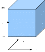
Cube de côté : \(L=2\)
1.3.2. Propriétés du matériau#
\(E=2N/{m}^{2}\)
\(\nu =0.\)
1.3.3. Conditions aux limites et chargements#
Déplacements imposés
plan \(z=\mathrm{1m}\) \(\mathrm{DX}=0.=\mathrm{DY}=0.=\mathrm{DZ}=0.\)
plan \(z=3m\) \(\mathrm{DZ}=\mathrm{2.m}\)
1.4. Solution de référence#
1.4.1. Méthode de calcul#
Le coefficient de poisson est nul \(\nu =0\) ce qui nous donne
\({\sigma}_{xx}={\sigma}_{yy}={\sigma}_{xy}={\sigma}_{xz}={\sigma}_{yz}=0\)
\({\sigma}_{zz}=E\epsilon =E\frac{\mathrm{DZ}}{L}\)
1.4.2. Résultats de référence#
\(\mathrm{SIZZ}=2N/{m}^{2}\) En tout point du cube